Data

A data set can often be viewed as a collection of data objects
Other names for a data object include recorde, point, vector, pattern, event, case, sample, observation or entity.
Data objects are described by a number of attributes that capture the basic charateristics of an object.
Other names for an attribute are variable, characteristic, field, featrue, or dimension.
A data set is usually a file, in which
- The objects are records in the file and
- Each field corresponds to an attribute.

Attribute

An attribute is a property or characteristic of an object to another or from one time to another
A mesasurement scale is a rule that associates a numerical or symbolic value with an attribute of an object.
The process of mesurement is the application of a measurement scale to associate a value with a particular attribute of a specific object.

Different types of attributes

There define four types of attributes

Nominal

Ordinal

Interval

Ratio

Nominal and orinal attributes are collectively referred to as categorical or quanlitative attributes.
Interval and ratio attributes are collectively referred to as quantitative or numeric attributes.

Nominal

values of a nominal attribute are just different names.
They provide only enough informatin ot distinguish one object from another.
Example: eye color, gender.

Ordinal

The values of an ordinal attribute provide enough information to odrder objects.
Example: grade

Interval

For interval attributes, the differences between values are meaningful.
Example: calendar dates.

Ratio

For ratio variables, both differences and ratios are meaningful
Example: monetaru quantities, mass, length
Another way to distinguish between attributes is by the number of values they can take.
Based on this criterion, attributes can be calssified as either discrete or continuous

Discrete

A discrete attribute has a finte or countably infinite set of values.
Such attributes can be categorical, such as gender, or numeric, such as counts.
Binary attributes are a special case of discrete attributes and assume only two values, e.g. true/false, yes/no, male/female, or 0/1

Continuous

A continuous attribute is one whose values are real numbers
Examples include temperature, height or weight.
Continuous attributes are typically represented as floating point variables.

Types of data sets

Following different types of data sets

Record data
Transacion or market basket data
Data matrix
Sparse data matrix

[]!()

Record data

A data set is usually represented as a coleection of records
Each record consists of a fixed set of data fields
Record data is usually stored eirher in flat files or in relational database.

Transaction or market basket data

Transaction data is a special type of record data.
Each transaction involves a set of items
Example: the set of products purchased by a customer during one shopping trip constitues a transaction.

Data matrix

If the data objects all have the same fixed set of numeric attributes, then they can be thought of as points in a multi-dimensional space.
This kind of data set can be interpreted as an m by n matrix where
- There are m rows, one for each object.
- There are n cols, one for each attribute.
Standard matrix operations can be applied to transform and mainipulate the data.

Sparse data matrix

A sparse data matrix is a special case of a data matrix in which there are a large number of zeros in the matrix, and only the non-zero attribute values are important
Sparsity is an advantage because usually only the non-zero values need to be stored and manipulated.
This results in significant savings with respect to computation time and storage.
An examlple is cocument data.
A document can be represented as a term vector, where
- Each term is a component of the vector and
- The value of each component is the number of times the corresponding term occurs in the document.
This representation of a coleection of documents is often called a document-term matrix.

Data quality

Precision
- The closeness of repeated measurements to ne another
- This is often measured by the standard deviation of a set of values.
Bias
- Asystematic variation of measurements from the quantity being measured.
- This is measured by takingthe differents between
  - the mean of the set of values and
  - the known value of the quantity being measured.
Suppose we have a standard laboratory weight with a mass of 1g.
We want to assess the precision and bias of our new laboratory scale.
We weight the mass five times, and obtain the values: {1.015, 0.990,1.013,1.001,0.986}
The mean of these values is 1.001
The bias is thus 0.001
The precision, as measured by the standard devation, is 0.013
Noise
- Noise is the random component of a measurement error.
Outliers
- Data objects that, in some sense, have characteristics that are different from most of the other data objects in the data set.
- Values of an attribute that are unusual with respect to the typical values of that attribute

Data quality: Missing values

It is not unusual for an object to be missing one or more attribute values.
There are several strategies for dealing with missing data
- Eliminate data object
- Estimate missing values
Eliminate data object
- If a data set has only a few objects taht have missing attribute values, then it may be convenient to omit them.
- However, even a partially specified data object contains some information.
- If many objects have missing values, then a reliable analysis can be difficult ot impossible
Estimate missing values
- A missing attribute value of a point can be estimated by the corresponding attribute values of the other points.
- If the attribute is discrete, then the most commonly occuring attribute value can be used.
- If the attribute is continuous, then the average attribute value of similar points is used.

Data preprocessing

There are a number of techniques for performing data preprocssing
- Aggregation
- Sampling
- Dimensionality reduction
- Discretization
- Normalization

Aggregation(聚合)

Aggreation is the combining of two or more objects into a single object.
There are several motivations for aggregation
- The smaller data sets resulting from agrreation require less memory and processing time.
- Aggregation can also provide a high-level view of the data
- Aggregate quantites, such as averages or totals, have less variability than the individual objects.
A disadvantage of aggregation is the potential loss of interesting details.

Sampling

Sampling is the selction of a subset of the data objects to be analyzed.
Sometimes, it is too expensive or time consuming to process all the data.
Using a sampling algorithm can reduce the data size to a point where a better, but more computationally expensive algorithm can be used.
A sample is representative if it has approximately the same property as the original set of data.
The simplest type of sampling is uniform random sampling.
For this type of sampling, there is an equal probability of seecting any particular item.
There are two variations on random sampling
- Sampling without replacement
- Sampling with replacement
Sampling without relacement
- As each item is selected, it is removed from the set of all objects.
Samepling with replacement
- Objects are not removed from the data set as they are selcted.
- The same object can be picked more than once.
Once a sampling technique has been selected, it is still necessary to choose the sample size.
For larger sample sizes
- The probaility that a sample will be representative will be increased.
- However, much of the advantage of sampling will also be eliminated.
For smaller sample sizes
- There may be a loss of important information

Dimensionality reduction

The dimensionality of a data set is the number of attributes that each object possesses.
It is usually more difficult to analyze high-dimensional data
An important preprocessing step is dimensionality reduction.
Dimensionality reduction has a number of advantages:
- It can eliminate irrelevant featrues and reduce noise.
- It can lead to a more understandable model which involves fewer attributes.
- It may allow the data to be more easily visualized.
- The amount of time and memory required for proessing the data is reduced.
The curse of dimensionality refers to the phenomenon that many types of data analysis become significantly harder as the number of dimensions increases.
As the number of dimensions increases, the data becomes increasingly sparse in the space that it occupies.
There may not be enoygh data objects to allow the reliable creation of a model that describes the set of objects.
There are a number of techniques for dimensionality reduction
- Feature transformation
- Feature subset selection
Feature transformation
- Feature transformation can be used to project data from a high-dimensional space to a low-dimensonal space.
- Principal Component Analysis(PCA) is a feature transformation technique to find new attriubtes that are
  - linear combinations of the original attributes.
  - capture the maximum amount of variation in the data.

Feature subset selection

Another way to reduce the number of dimentsions is to use only a subset of the features.
This approach is effective if redundant and irrelevant fetures are present.
Redundant features duplicate much or all of the information contained in one or more other attributes.
Irrelevant features contain almost no useful information for the task at hand.
The ideal approach to feature selection is to
- Try all possible subsets of freatures
- Take the subset that produces the best result
Since the number of subsets involving n attributes is 2^n, such an approach is impractical in most situations
There are three standard approaches to feature selection
- Embedded approaches
- Filter approaches
- Wrapper approaches

Embedded approaches

Feature selection occurs naturally as part of the algorithm
The algorithm itself decides which attributes to use and which to ignore

Filter approaches

Features are selected before the algorithm is run
An evaluation measure is used to determine the goodness of a subset of attributes
This measure is independent of the current algorithm used

Wrapper approaches

These methods use the target algorithm as a black box to find the best subset of attributes.
Typically, not all the possible subsets are considered

Discretization

In some cases, we prefer to use data with discrete attributes
It is thus necessary to transform a continous attribute into a discrete attribute
Transformation of a continuous attribute to a discrete attribute involves two subtasks
- Deciding how many possible discrete values to have
- Determining how to map the values of the continuous atrribute to these discrete values
In the first step
- The values of the coninuous attribute are first sorted
- They are then divided into S intervals by specifying S-1 split points
In the second step
- All the values in one interval are mapped to the same discrete value

Normalization

The goal of normalization or standardization is to make an entire set of values have a particular property
Normalization is necssary to avoid the case where a variable with large values dominates the result of the calculation

Similarity and dissimilarity

The similarity between two objects is a numerical measure of the degree to which the two objects are alike
Similarities are higher for pairs of objects that are more alike
The dissimilarity between two objects is a numerical measure of the degree to which the two objects are different
Dissimilarityes are lower for more similar pairs of objects
Freuently, the term distance is used as a synonym for dissimilarity
The term proximity is used to refer to either similarity or dissimilarity

Dissimilarity between attribute values

We consider the definition of dissimilarity measures for the following attribute types
- Nominal
- Ordinal
- Intervale/Ratio

Nominal

Nominal attributes only convey information about the distinctness of objects
All we can say is that two objects either have the same attribute value or not
As a result, dissimilarity is defined as
- 0 if the attribute avlues match
- 1 otherwise

Ordinal

For ordinal attributes, information about order should be taken into account
The values of the ordinal attribute are often mapped to successive integers
The dissimilarity can be defined by taking the absolute difference between these integers

Interval/Ratio

For interval or ratio attributes, the natural measure of dissimilarity between two objects is the absolute differece of their values

Distance

The Euclidean distance d between two points x and y is given by

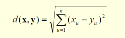
n is the number of dimensions
Xu and Yu are, respectively, the u-th attributes of x and y
The Euclidean distance measure is generalized by the Minkowski distance metric as follows:

Three most common examples of Minkowski distances are
- h=1: City block distance(L1 norm)
- h=2: Euclidean distance(L2 norm)
- h=00: Supremum distance(Lmax norm), which is the maximum difference between any attribute of the objects
A distance measure has some well-known properites
- Positivity
  - d(x,y)>=0 for all x and y
  - d(x,y)=0 if and only if x =y
- Symmetry
  - d(x,y)=d(y,x) for all x and y
- Triangle inequality
  - d(x,z)<=d(x,y)+d(y,z) for all points x,y,z
all attributes were treated eually when computing the distance
This is not desirable when some attributes are more important than others
To address these situations, the distance measure can be modified by weighting the contribution of each attribute:

Summary statistics

Summary statisticss are quantities that capture various characterics of a large set of values using a small set of numbers
We consider the following summary statistics
- Relative frequency and the mode
- Measure of location: mean and meadian
- Measure of spread: range and variance

Realtive frequency and the mode

Suppose we are given a discrete attribute x, which can take values{a1,..,as,...,as}, and a set of m objects
The relative frequency of a value as is defined as

The mode of a discrete attribute is the value that has the highest relative frequency

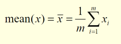
Mean

We consider a set of m objects and an attribute x
Let {x1,...,xm} be the attribute values of x for these m objects
The mean is defined as follows:

Median

Let{x1,...,xm} represent the values of x after they have been sorted in non-decreasing order
Thus, x1= xmin and xm = xmax
The meadian is defined as follows:

Mean and Median

The mean is sensitive to hte presence of outliers
The median provides a more robust numerical summary of a set of values
To overcome problems with the mean, the notion of a trimmed mean is sometimes used.
- A percentage p between 0 and 100 is specified
- The top and bottom (p/2)% of the data is thrown out
- The mean is then calculated in the normal way

Range

The simplest measure of spread is the range
Given an attribute x with a set of m values{x1,...,xm}, the range is defined as

However, using the range to measure the spread can be misleading if
- most of the values are concentrated in a narrow band of values
- there are also a relatively small number of more extreme values

Variance

The variance of the values of an attribute x is defined as follows:

The standard deviation, which is the square root of the variance, is denoted as

Multivariate summary statistics

The mean or median of a data set that consists of several attributes can be obtained by computin the mean or median separately for each attribute
Given a data set, the mean of the data objects is given by :
For multivariate data, the spread of the data is most commonly captured by the covariance matrix C.
The uv-th entry Cuv is the covariance of the u-th and v-th attributes of the data.
This covariance is given by
The covariance of two attributes is a measure of the degree to which two attributes vary together
this measure depends on the magnitudes of the variables
In view of this, we perform the following operation on the covariance to obtain the correlation coeffient ruv.
are the standard deviations of xu and xv respectively
The range of ruv is form -1 to 1

Data visualization

The motivation of using data visualization is that people can quickly absorb large amounts of visual information and find patterns in it.
We consider the following data visualizaiton techniques
- Histogram
- Scatter plot

Histogram

A histogram is a plot that displays the distribution of attribute values by
- dividing the possible values into bins and
- showing the number of objects that fall into each bin
Each bin is represented by one bar
The area of each bar is proportional to the number of values that fall into the corresponding range

Scatter plot

A scatter plot can graphically show the realtionship between two attributes.
In particular, it can be used to judge the degree of linear correlation of the attributes.