CS3481-Lecture-3
Decision Tree
Classification
Basic Concept
Classification is the task of assigning objects to one of several predefined categories
It is an important problem in many applications
- Detecting spam email messages based on the message header and content
- Categorizing cells as malignant or benign based on the results of MRI scans
- Classifying galaxies based on their shapes
The input data for a classification task is a collection fo records
Each record, also known as an instance or example, is characterized by a tuple(x,y)
- x is the attribute set
- y is the class label, also known as category or target attribute.
The class label is a discrete attribute.
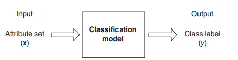
Classification is the task of learning a target function f that maps each attribute set x to one of the predefined class labels y.
The target function is also known as a classification model.
A classification model is useful for the following purposes
- Descriptive modeling
- Predictive modeling
A classification technique is a systematic approach to perform classification on an input data set
Example include
- Decision tree classifiers
- Neural networks
- Support vector machines
General Framework for Classification
A classifcation technique employs a learning algorithm to identify a model that best fits the relationship between the attribute set and the class label of the input data.
The model generated by a learning algorithm should
- Fit the input data well and
- Correctly predict the class labels of records it has never seen before
A key objective of the learning algorithm is to build models with good generalization capability.
First, a training set consisting of records whose class labels are known must be provided.
The training set is used to build a classification model.
This model is subsequently applied to the test set, which consists of records which are different from those in the training set.

Confusion matrix
Evaluation of the performance of the model is based on the counts of correctly and incorrectly predicted test records.
These counts are tabulated in a table known as a confusion matrix
Each entry aij in this table denotes the number of records from class i predicted to be of class j.
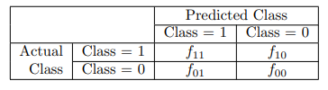
The total number of correct predictions made by the model is f11 + f00
The total number of incorrect predictions is f10+f01
The information in a confusion matrix can be summarized with the following two measures
- Accuracy

in binary that is
- Error rate
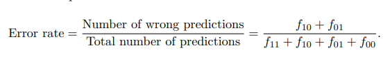
- Accuracy
Most classification algorithms aim at attaining the highest accuracy, or equivalently, the lowest error rate when applied to the test set.
Decision tree construction
Concept
We can solve a classification problem by asking a series of carefully crafted quesions about the attributes of the test record.
Each time we receive an answer, a follow-up question is asked.
This process is continued until we reach a conclusion about the class label of the record.
The series of questions and answers can be organized in the form of a decision tree.
It is a hierarchical structure consisting of nodes and directed edges.
The tree has three types of nodes
- A root node that has no incoming edges.
- Internal nodes, each of which has exactly one incoming edge and a number of outgoing edges.
- Leaf or terminal nodes, each of which has exactly one incoming edge and no outgoing edges.
In a decision tree, each leaf node is assigned a class label.
The non-terminal nodes, which include the root and other internal nodes, contain attribute test conditions to separate records that have different charaacteristics.
Classifying a test record is straightforward once a decision tree has been constructed.
Starting from the root node, we apply the test condition
We then follow the appropriate branch based on the outcome of the test
This will lead us either to
- Another internal node, at which a new test condition is applied, or
- A leaf node
The class label associated with the leaf node is then assigned to the record.

Effient algorithms have been developed tot induce a reasonably accurate, although suboptimal, decision tree in a reasonable amount of time.
These algorithms usually employ a greedy strategy that makes a series of locally optimal decisions about which attribut to use for partitioning the data.
Hunt’s Algorithm
A decision tree is grown in a recursive fashion by paritioning the training records into successively purer subsets
We suppose
- Us is the set of training records that are associated with node s.
C={c1,c2,..,ck}is the set of class labels.
If all the records in Us belong to the same class ck, then s is a leaf node labeled as ck.
If Us contains records that belong to more than one class,
- An attribute test condition is selected to parition the records into smaller subsets.
- An child node is created for each outcome of the test condition.
- The records in Us are distributed to the children based on the outcome.
The alogirithm is then recutsively appled to each child node.
For each node, let p(ck) denotes the fraction of training records from class ck
In most cases, the leaf node is assigned to the class that has the majority number of training records.
The fraction p(ck) for a node can also be used to estimate the probability that a record assigned to that node belongs to class k.
Decision trees that are too large are susceptible to a phenomenon known as overfitting.
A tree pruning step can be performed to reduce the size of the decision tree.
Pruning helps by trimming the tree branches in a way that improves the generalization error.
Attribute Test
Each recursive step of the treee-growing process must select an attribute test condition to divide the records into smaller subsets.
To implement this step, the algorithm must provide
- A method for specifying the test condition for different attribute types and
- An objective measure for evaluating the goodness of each test condition.
Binary attribute
- The test condition for a binary attribute generates two possible outcomes

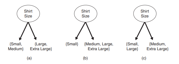
Nominal attributes
- A norminal attribute can produce binary or multi-way splits.
- Thereare 2^(s-1)-1 ways of creating a binary partition of S attribute values.
- For a multi-way split, the number of outcomes depends on the number of distinct values for the corresponding attribute.
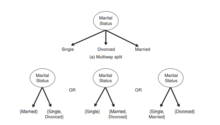
Ordinal attributes
- Ordinal attributes can also produce binary or multi-way splits.
- Ordinal attributes can be grouped as long as the grouping does not violate the order property of the attribute values.
Continuous attributes
- The test condition can be expressed as a comparison test x<=T pr x > T
- For the binary case
- The decision tree algorithm must consider all possible split positions T, and
- Select the one that produces that best partition
- For the multi-way split
- The algorithm must consider multiple split positions.

- The algorithm must consider multiple split positions.
conduction example
We consider the problem of using a decision tree to predict the number of participants in a marathon race requiring medical attention.
This number depends on attributes such as
- Temperature forecase (TEMP)
- Humidity forecast (HUMID)
- Air pollution forecast (AIR)
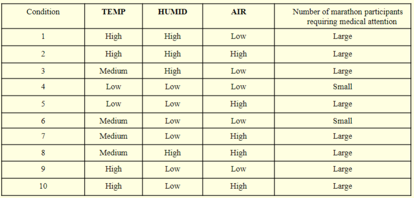
In a decision tree, each internal node represents a particular attribute, e.g. TEMP or AIR
Each possible value of that attribute coresponds to a branch of the tree.
Leaf nodes represent classifications, such as Large or Small number of participants requiring medical attention.

Suppose AIR is selected as the first attribute.
This partitions the examples as follows.

Since the entries of the set
{2,5,7,8,10}all coreespond to the case of a large number of participants requiring medical attention, a leaf node is formed.On the other hand, for the set
{1,3,4,6,9}- TEMP is selected as the next attribute to be tested.
- This further divides this partition into
{4}, {3,6} and {1, 9}
Information theory
Concept
Each attribute reduces a certain amount of uncertainty in the classification process.
We calcualte the amount of uncertainty reduced by the selection of each attribute.
We then select the attribute that provides the greatest uncertanty reduction.
Information theory provides a mathematical formulation for measuring how much information a message contains.
We consider the case where a message is selected among a set of possible messages and transmitted.
The information content of a message depends on
- The size of this message set, and
- The frequency with which each possible message occurs.
The amount of information in a message with occurrence probability p is defined as -log2p.
Suppose we are given
- a set of messages,
C={c1,c2,...,ck} - the occurrence porbality p(ck) of each ck.
- a set of messages,
We define the entropy I as the expected in formation content of a message in C:
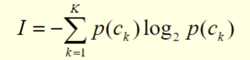
The entropy is measured in bits.
Attribute selection
We can calcualte the entropy of a set of training examples from the occurrence probabilities of the different classes.
In our example
- p(Small) = 2/10
- p(Large) = 8/10
The set of training instances is denoted as U
We can calculate the entropy as follows:

The information gain provided by an attribute is the difference between
- The degree of uncertainty before including the attribute
- The degree of uncertainty after including the attribute.
Item 2 above is defined as the weighted average of the entropy values of the child nodes of the attribute.
If we select attribute P, with S values, this will partition U into the subsets {U1,U2,…,Us}.
The average degree of uncertainty after selectin P is

The information gain associated with attribute with attribute P is computed as follows.

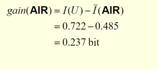
If the attibute AIR is chosen, the examples are partitioned as follows:
U1={1,3,4,6,9}U2={2,5,7,8,10}
The resulting entropy value is

The information gain can be computed as follows:
For the atttribute TEMP which partitions the examples into
U1 = {4,5},U2={3,6,7,8}andU3={1,2,9,10}:
For the attribute HUMID which partitions the examples into
U1={4,5,6,7,9,10}andU2={1,2,3,8}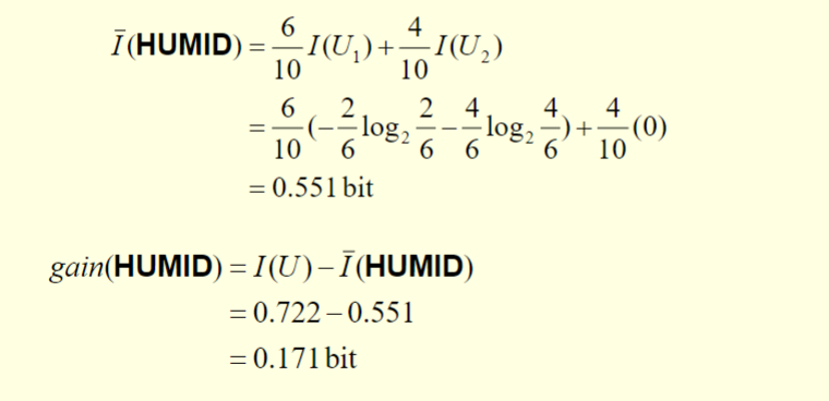
The attribute AIR correcsponds to the highest information again.
As a result, this attribute will be selected.
Continuous attributes
If attribute P is continuous with value x, we can apply a binary test.
The outcome of the test depends on a threshold value T.
There are two possible outcomes:
- x <=T
- x > T
The traning set is then partitioned into 2 subsets U1 and U2.
We apply sorting to values of attribute P to abtain the sequence
{x1,x2,...,xm}Any threshold between xr and x(r+1) will divide the set into two subsets
{x1,x2,...,xr}{x(r+1),x(r+2),...,xm}
There are at most m-1 possible splits.
For r = 1,…,m-1 such that x(r) != x(r+1), the corresponding threshold is chosen as Tr=(x(r)+x(r+1))/2
We can then calculate the information gain for each Tr

- where I(P,Tr) is a function of Tr
The threshold Tr which maximizes gain(P,Tr) is then chosen.
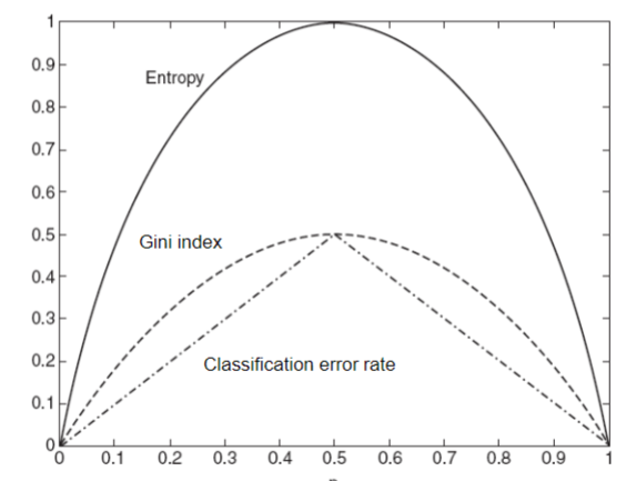
Impurity measures
The measures developed for selecting the best split are often based on the degree of impurity of the child nodes.
Besides entropy, other examples of imputrity measures include
- Gini index
- Classification error rate
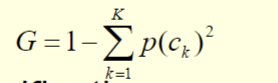
- Gini index
In the following figure, we compare the values of the imputrity measures ofr binary classification problems.
p refers to the fraction of records that belong to one of the two classes
All three measures attain their maximum value when p = 0.5
Then minimum values of the measures are attained when p equals 0 or 1

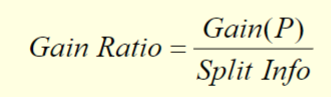
Gain ratio
Impurity measures such as entropy and Gini indesx tend to favor attributes that have a large number of possible values.
In many cases, a test condition that results in a large number of outcomes may not be desirable
This is because the number of records associated with each partition is too small to enable us to make any reliable predictions.
To solve this problem, we can modify the splitting criterion to take into account the number of possible attribute values.
In the case of informatoin agin, we can use the gain ratio which is defined as follows
where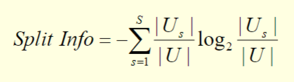
Oblique decision tree
The test condition described so far involve using only a single attribute at a time
The tree-growing procedure can be viewed as the process of partitioning the attribute sapce into disjoint regions.
The border between two neighboring regins of different classes is known as a decisionboundary.
Since the test condition involves only a single attribute, the decision boundaries are parallel to the coordinate axes.
This limits the expressiveness of the decision tree representation for modeling complex relationships among continuous attributes.

An oblique decision tree allows test conditions that involve more than one attribute
The following figure illustrates a data set that connot be classified effectively by a conventional decision tree
This data set can be easily represented by a single node of an oblique decision tree with the test condition x+y<1
However, finding the optimal test condition for a given node can be computationally expensive.
