CS3103-Lecture-4
Scheduling
why Scheduling is Needed?
Maximum CPU utilization
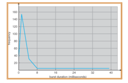
- CPU-I/O Burst Cycle: Process execution consists of a cycle of CPU execution and I/O wait
- CPU burst distribution
- Alternating Sequence of CPU and I/O Burst
Do multiple tasks concurrently
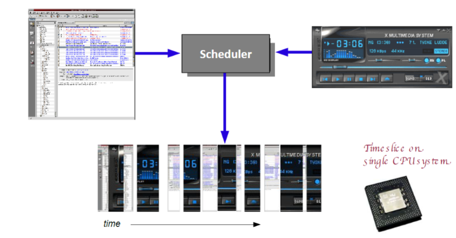
Scheduler
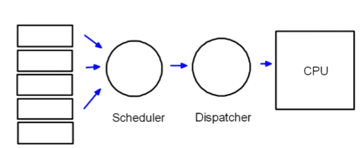
CPU Scheduler(Short-term Scheduler)
- Selects from among the tasks in memory that are ready to execute, and allocates the CPU to one of them
- CPU scheduling decisions may take place when a task
- Switches from running to waiting state
- Switches from running to ready state
- Switches from waiting to ready
- Terminates
Dispatcher
- Dispatcher module gives control of the CPU to the task selected by the short-term scheduler; this involves:
- switching context
- switching to user mode
- jumping to the proper location in the user program to restart that program
- Dispatch latency - time it takes for the dispatcher to stop one task and start anohter running
Scheduling Criteria
- CPU utilization - keep the CPU as busy as possible => we want to maximize
- Throughput - of tasks that complete their execution per time unit => we want to maximize
- Waiting time - amount of time a task has been waiting in the ready queue => we want to minimize
- Turnaround time - time takes from when a request was submitted until the task is finished => we want to minimize
- Response time - time takes from when a request was submitted until the start of its execution => we want to minimize
Scheduling Policy
An algorithm used for distributing resources among parties which simultaneously and asynchronously request them
- In the context of CPU scheduling, an alogorithm decides which task to execute on CPU at which time
Many scheduling policies
- First-Come First-Served (FCFS)
- Shortest-Job-First (SJF)
- Round Robin (RR)
- Priority Scheduling
First-Come First-Served(FCFS)
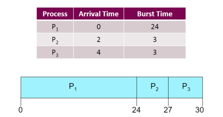
Waiting time for P1=0; P2 = 22; P3 = 23
Average waiting time: (0+22+23)/3 = 15
Suppose that the processes all arrive at time 0, but in the order
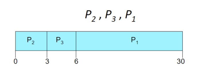
Waiting time for P1 = 6; P2= 0; P3=3
Average waiting time: (6+0+3)/3 = 3
Shortest-Job-First(SJF)
- Schedule the process with the shortest length of its next CPU burst time(execution time)
- Two schemes:
- nonpreemptive - once CPU given to a process, it cannot be preempted until completes its CPU burst
- preemptive - if a new process arrives with CPU burst length less than remaining time of current executing process, preempt. This scheme is also known as the Shortest-Remaining-Time-First(SRTF)
- SJF is optimal regarding average waiting time
Non-Preemptive SJF

- Average waiting time = (0+6+3+7)/4 = 4
Preemptive SJF

- Average waiting time = (9+1+0+2)/4 = 3
Determining Length of Next CPU Burst
- We can only estimate the length of future CPU bursts
- Can be done by using the length of previous CPU bursts
- For example, exponential averaging
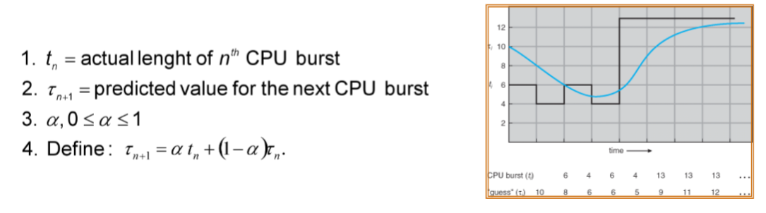
- For example, exponential averaging
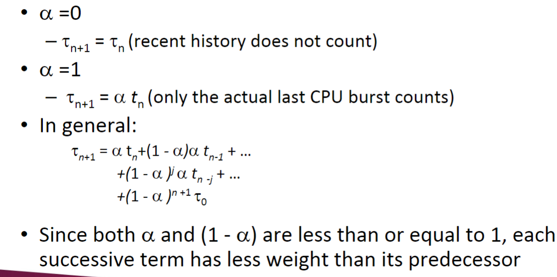
Examples of Exponential Averaging
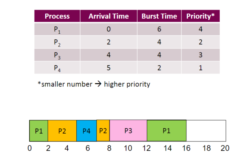
Priority Scheduling
A priority number is associated with each task
The CPU is allocated to the task with the highest priority(usually, smallest integer <- -> highest priority)
- Preemptive or Nonpreemptive
SJF is a priority scheduling where priority is the CPU burst time
Example of Priority Scheduling
Round Robin(RR)
Each task gets a small unit of CPU time(time quantum)
- Typically 10-100 milliseconds
- Once elapsed, preempted and added to the end of the ready queue
If there are n tasks and the time quantum is q, the each process gets 1/n of the CPU time in chunks of at most q time units at once
- No task waits more than (n-1)q time units
Performance
- q large => slow responsiveness
- q small => high context switch overhead
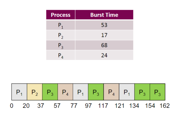
Example of RR with Time Quantum = 20
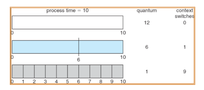
Time Quantum and Context Switch Overhead
- If the time quantum is extrmely large, the RR policy is the same as the FCFS policy
- If the time quantum is small, high context switch overhead
- The time quantum must be much larger than context switch overhead
- The time quantum must be much larger than context switch overhead
Turnaround Time Varies With Time Quantum
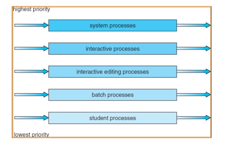
Multilevel Queue
Ready queue is paritioned into separate queues e.g.,
- foreground (interactive applications)
- backgound (batch applications)
Each queue has its own scheduling algorithm, e.g.,
- foreground - RR
- background - FCFS
Scheduling must be don between the queues
- Fixed priority(i.e., serve all from foreground then from background)
- Time slice - each queue gets a certain amount of CPU e.g., 80% to foreground in RR and 20% to backgournd in FCFS
For example, 5-level queues
Multilevel Feedback Queue
- A task can move between the various queues
- Multilevel-feedback-queue scheduler defined by
- number of queues
- scheduling algorithms for each queue
- method used to determine when to upgrade a task
- method used to determine when to demote a task
- method used to determine which queue a task will enter when that task needs service
- Flexible yet complex algorithms to implement
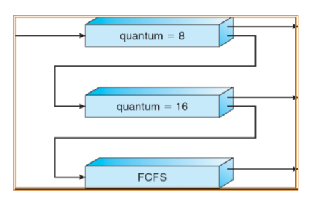
Example of Multilevel Feedback Queue
Three queues
- Q0 - RR with time quantum 8 milliseconds
- Q1 - RR with time quantum 16 milliseconds
- Q2 - FCFS
Scheduling
- A new task enters queue Q0. When it gains CPU, task receives 8 milliseconds. If it does not finish in 8 milliseconds, moved to queue Q1
- If it still does not complete in Q1, it is preempted and moved to queue Q2
Exmaple: CPU Scheduling in Linux(2.6.23)
Scheduling classes
- Default: scjeduled by Completely Fair Scheduler(CFS)
- Real-Time:scheduled according to priority
- (other classes can be added)
Read-time tasks have priority over CFS tasks
Completely Fair Scheduler(CFS)
- Rather than quantum based on fixed time allotments, based on proportion of CPU time(nice value)
- Nice value from -20 ot +19
- Larger nice values correspond to a lower priority
- you are “nice” to the other processes
- Rather than quantum based on fixed time allotments, based on proportion of CPU time(nice value)
Maintains task virtual run time
- Associate with decay factor based on nice value
- Larger nice value is higher decay rate
- Normal default nice value (0) yields virtual run time = actual run time
- Associate with decay factor based on nice value
Scheduler picks the task with lowest virtual run time to run next