CS3481-Lecture-4-Classifier Evaluation

Classification error

• The errors committed by a classification model are generally divided into two types

  • Training errors
  • Generalization errors

• Training error is the number of misclassification errors committed on training records

• Training error is also known as resubstitution error of apparent error.

• Generalization error is the expected error of the model on previously unseen records.

• A good classification model should

  • Fit the training data well.
  • Accurately classify reocrds it has never seen before.

• A model that fits the training data too well can have a poor generaliztion error.

• This is known as model overfitting

• We consider the 2-D data set in the following figure.

• The data set contains data points that belong to two different calsses.

• 10% of the points are chosen for training, while the remaining 90% are used for testing.

• Decision tree calssifiers with different numbers of leaf nodes are built using the training set.
  

• The following figure shows the training and test error rates of the decision tree.

• Both error rates are large when the size of the tree is very small.

• This situation is known as model underfitting.

• Underfitting occurs because the model cannot learn the true structure of the data.

• It performs poorly on both the training and test sets.
  

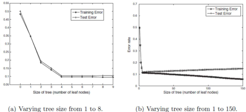
• When the tree becomes too large

  • The training error rate continues to decrease
  • However, the test error rate begins to increase.

• This pheonmenon is known as model overfitting

Overfitting

• The training error can be reduced by increasing the model complexity

• However, the test error can be large because the model may accidentally fit some of the noise point in the training data.

• In ohter words, the performance of the model on the training set does not generalize well to the test examples.

• We consider two decision treews, one with 5 leaf nodes and one with 50 leaf nodes.

• The two decision trees and their corresponding decision boundaries are shown in the following figures.
  
  

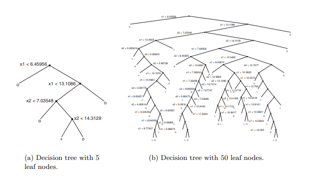
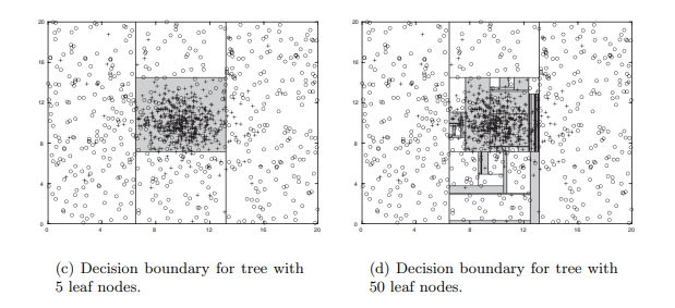
• The decision boundaries constructed by the tree with 5 leaf nodes represent a reasonable approximation of the optimal solution.

• It is expected that this set of decision boudnaries will result in a good classification performance on the test set.

• On the other hand, the tree with 50 leaf nodes generates a set of complicated decision boundaries.

• Some of the shaded regions corresponding to the ‘+’ class only contain a few ‘+’ training instances, among a large number of surrounding ‘o’ instance.

• This excessive fine-tuning to specific patterns in the data will lead to unsatisfactory classification performance on the test set.

Generalization error estimation

• The ideal classification model is the one that produeces the lowest generalization error.

• The problem is that the model has no knowledge of the test set.

• It has access only to the training set.

• We consider the following approaches to estimate the generalization error

  • Resubstitution estimate
  • Estimates incorporating model complexity
  • Using a validation set

Resubstitution estimate

• The resubstitution estimate approach assumes that the training set is a good representation of the overall data

• However, the training error is usually an optimistic estimate of the generalization error.

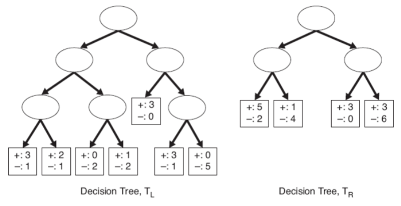
• We consider the two decision trees shown in the following figure.

• The left tree TL is more complex than the right tree TR.

• The training error rate for TL is e(TL) = 4/24 = 0.167

• The training error rate for TR is e(TR) = 6/25 = 0.24

• Based on the resubsitution estimate, TL is considered better than TR.
  

Estimates incorporating model complexity

• The chance for model overfitting increases as the model becomes more complex.

• As a result, we should prefer simpler models

• Based on this principle, we can estimate the generalization error as the sum of

  • Training error and
  • A penalty term for model complexity

• We consider the previous two decision trees TL and TR

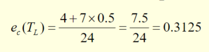
• We assume that the penalty term is equal to 0.5 for each leaf node.

• The error rate estimate for TL is:
  

• The error rate estimate for TR is:
  

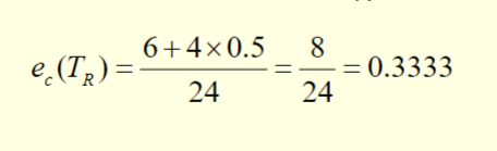
• Based on this penalty term, TL is better than TR

• For a binary tree, a penalty term of 0.5 means that a node should always be expanded into its two child nodes if it improves the classification of at least one training record.

• This is bcecause expanding a node, which is the same as adding 0.5 to the overall error, is less costly than committing one training error.

• Suppose the penalty term is equal to 1 for all the leaf nodes

• The error rate estimate for TL becomes 0.458

• The error rate estimate for TR becomes 0.417

• So TR is better than TL

• A penalty term of 1 measns that, for a binary tree, a node should not be expanded unless it reduces the classification error by more than one training record.

Using a validation set

• In this approach, the original training data is divided into two smaller subsets.
• One of the subsets is used for training
• Another one known as the validation set, is used for estimating the generalization error.
• This approach can be used in the case where the complexity of the model is determind by a parameter
• We can adjust the parameter until the resulting model attains the lowest error on the validation set.
• This approach provides a better way for estimating how well the model performs on previously unseen records.
• However, less data are available for training

Handling overfitting in decision tree

• There are two approaches for avoiding model overfitting in decision tree
  • Pre-pruning
  • Post-pruning

Pre-pruning

• In this approach, the tree growing algorithm is halted before generating a fully grown tree that perfectly fits the training data.
• To do this, an alternative stopping condition could be used
• For example, we can stop expanding a node when the observed change in impurity measure falls below a certain threshold.
• Advantage:
  • avoids generating overly compelx sub-trees that overfit the training data
• However, it is difficult to choose the right threshold for the change in impurity measure.
• A threshold which is:
  • too high will result in underfitted models
  • too low may not be sufficient to overcome the model overfitting problem

Post-pruning

• In this approach, the decision tree is initially grown to its maximum size
• This is followed by a tree pruning step, which trims the fully grown tree.
• Trimming can be done by replacing a sub-tree with a new leaf node whose class label is determined from the majority class of records associated with the node
• The tree pruning step terminates when no further improvement is observed
• Post-pruning tends to give better results than pre-pruning because it makes pruning decisions based on a fully grown tree.
• On the other hand, pre-pruning can suffer from prematrue termination of the tree growing process.
• However, for post-pruning, the additional computations for growing the full tree may be wasted when some of the sub-trees are pruned.

Classifier evaluation

• There are a number of methods to evaluate the performance of a classifier
  • Hold-out method
  • Cross validation

Hold-out method

• In this method, the original data set is partitioned into two disjoint sets.
• These are called the training set and test set respectively.
• The classification model is constructed from the training set.
• The performance of the model is evaluted using the test set.
• The hold-out method has a number of well known limitations.
• First, fewer examples are available for training.
• Second, the model may be highly dependent on the composition of the training and test sets.

Cross validation

• In this approach, each record is used the same number of times ofr training, and exactly once for testing.
• To illustrate this method, suppose we partition the data into two equal-sized subsets.
• Frist, we choose one of the subsets for training and the other for testing
• We then swap the roles of the subsets so that the previous training set becomes the test set, and vice versa.
• The estimated error is obtained by averaging the errors on the test sets for both runs.
• In this example, eachrecord is used exactly once for training and once for testing.
• This approach is called two-fold cross-validation
• The k-fold cross validation method generalizes this approach by segmenting the data into k equal-sized partitions.
• During each run
  • One for the partitions is chosen for testing
  • The rest of them are used for training
• This procedure is repeated k times so that each partition is used for testing exactly once.
• The estimated error is obtained by averaging the errors on the test sets for all k runs.