Hierarchical clustering

A hierarchical clustering is a set of nested clusters that are organized as a tree.
There are two basic approaches for generating a hierarchical clustering
- Agglomerative
- Divisive
In agglomerative hierarchical clustering, we start with the points as individual clusters.
At each step, we merge the closest pair of clusters.
This requires defining a notion of cluster distance
In divisive hierarchical clustering, we start with one, all-inclusive cluster
At each step, we split a cluster
This process continues until only singleton clusters of individual points remain
in this case, we need to decide
- Which cluster to split at each step and
- How to do the splitting
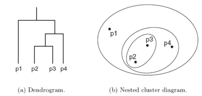
A hierarchical clustering is often displayed graphically using a tree-like diagram called the dendrogram
The dendrogram displays both
- the cluster-subcluster relationships and
- the order in which the clusters are merged(agglomerative) or split (divisive)
For sets of 2-D points, a hierarchical clustering can also be graphically represented using a nested cluster diagram.
The basic agglomerative hierarchical clustering algorithm is summarized as follows
- Compute the distance matrix
- Repeat
  - merge the closest two clusters
  - Update the distance matrix to reflect the distance between the new cluster and the original clusters.
- Until only one cluster remains
Different definitions of cluster distance leads to different versions of hierarchical clustering
These versions include
- Single link or MIN
- Complete link or MAX
- Group average
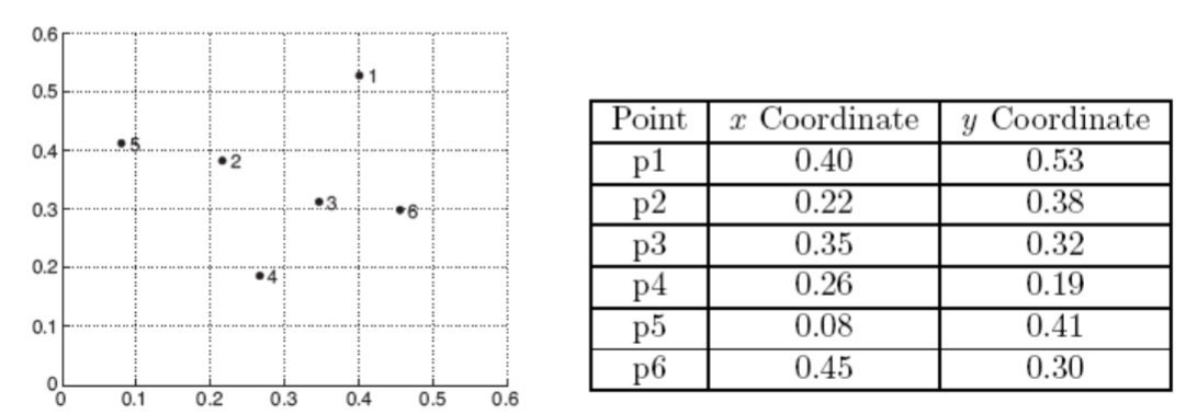
We consider the following set of data points.
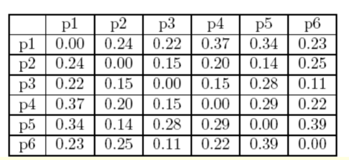
The Euclidean distance matrix for these data point is shown in the following slide.

Single Link

We now consider the single link or MIN version of hierarchical clustering
In this case, the distance between two clusters is defined as the minimum of the distance between any two points, with one of the points in the first cluster, and the other point in the second cluster
This technique is good at handling clusters with non-elliptical sahpes
The following figure shows the result of applying the single link technique to our example data.
The left figure shows the nested clusters as a sequence of nested ellipses.
The numbers associated with the ellipes indicate the order of the clustering.
The right figure shows the same information in the form of a dendrogram
The height at which two clusters are merged in the dendrogram reflects the distance of the two clusters.
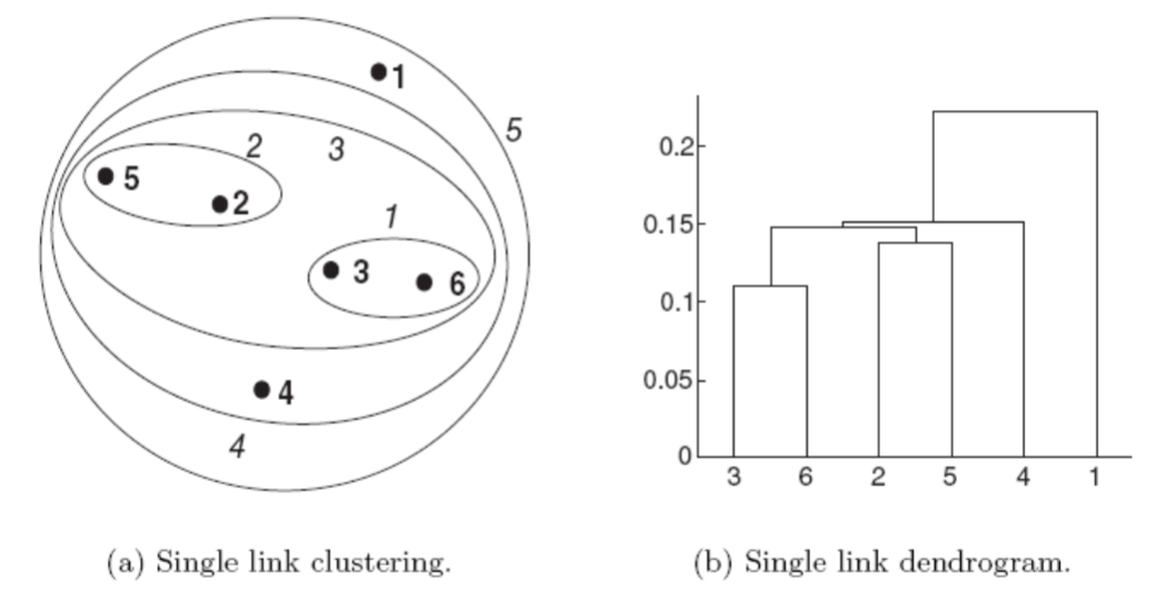
For example, we see that the distance between points 3 and 6 is 0.11
That is the height at which they are joined into one cluster in the dendrogram.
As another example, the distance between clusters {3,6}and {2,5} is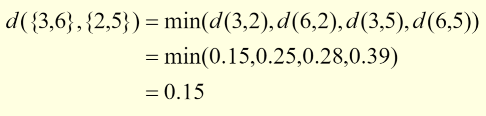

Complete Link

We now consider the complete link or MAX version of hierarchical clustering.
In this case, the distance between two clusters is defined as the maximum of the distance between any two points, with one of the points in the first cluster, and the other point in the second cluster
Complete link tends to produce clusters with globular shapes
The following figure shows the results of applying the complete link to our sample data points.
As with single link, points 3 and 6 are merged first.
Points 2 and 5 are then merged
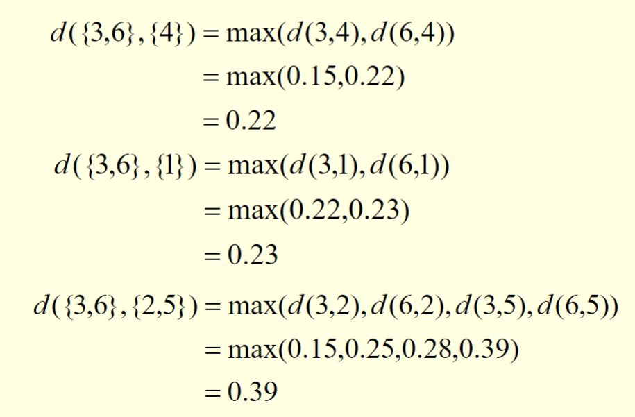
After that, {3,6} is merged with {4}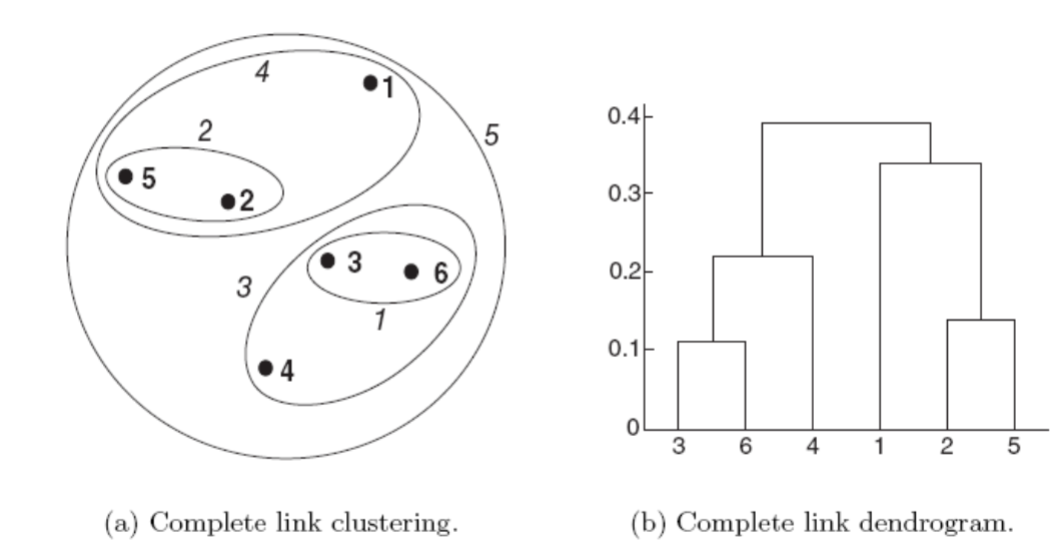
this can be explained by the following calculations

Group average

We now consider the group average version of hierarchical clsutering
In this case, the distance between two clusters is defined as the average distance across all pairs of points, with one point in each pair belonging to the first cluster, and the other point of the pair belonging to the second cluster.
This is intermediate approach between the single and complete link approaches.
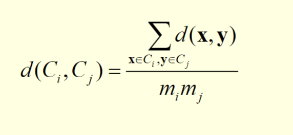
We consider two clusters Ci and Cj, which are of sizes mi and mj respectively
The distance between the two clusters can be expressed by the following equation
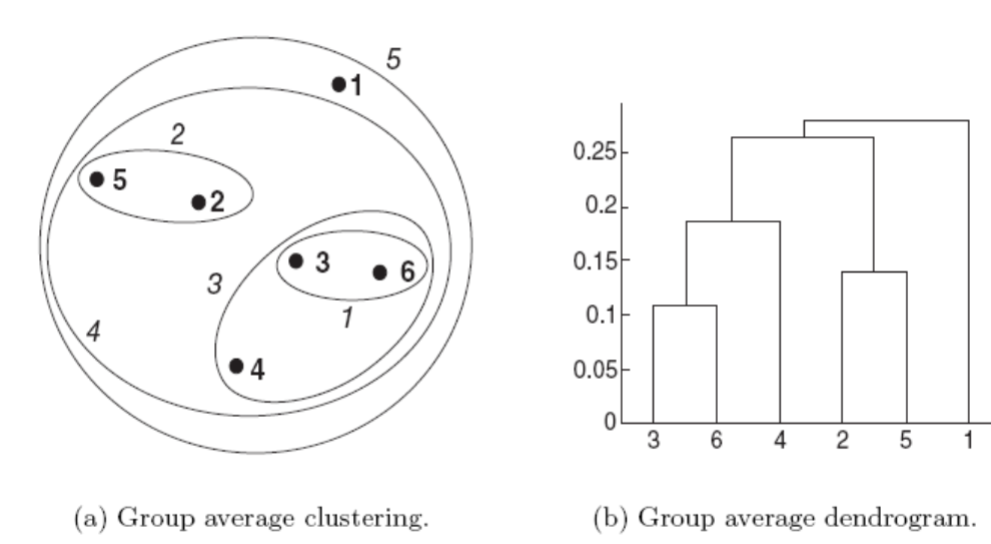
The following figure shows the results of applying the group average to our sample data
The distances between some of the clusters are calculated as follows:
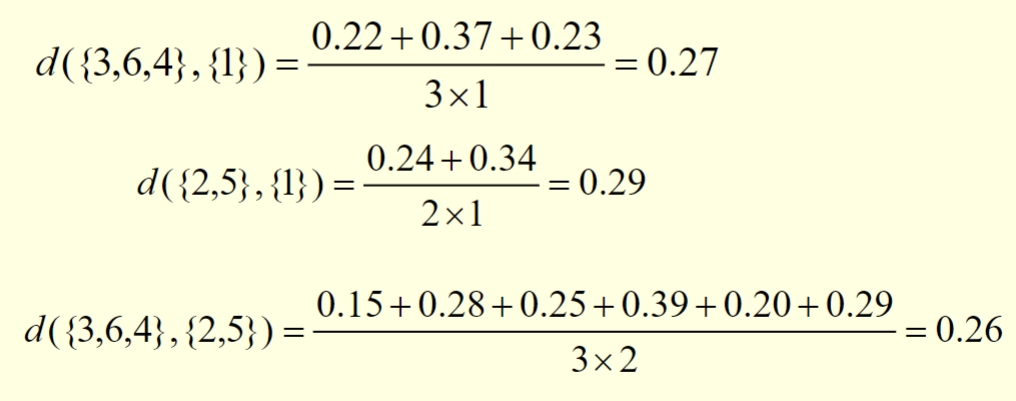
We observe that d({3,6,4},{2,5}) is smaller than d({3,6,4},{1}) and d({2,5},{1}).
As a result, {3,6,4} and {2,5} are merged at the fourth stage.

Key issues

Hierarchical clustering is effective when the underlying application requires the creation of a multi-level structure.
However, they are expensive in terms of their computational and storage requirements.
In addition, once a decision is made to merge two clusters, it cannot be undone at a later time.

DBSCAN

Density-based clustering locates regions of high density that are separated from one another by regions of low density.
DBSCAN is a simple and effective density-based clustering algorithm.
In DBSCAN, we need to estimate the density for a particular point in the data set.
This is performed by counting the number of points within or at a specified radius, Eps, of that point.
The count includes the point itself.
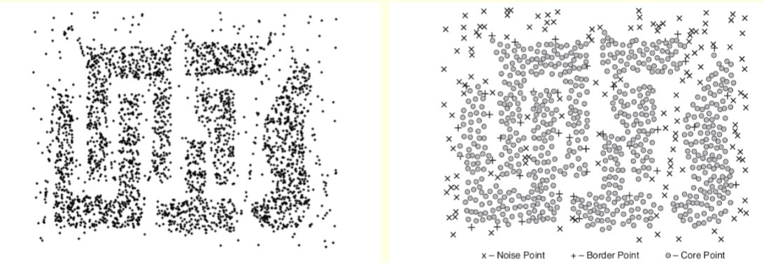
This technique is illustrated in the following figure.
The number of points within or at a radius of Eps of point A is 7, including A itself.
The density of any point will depend on the specified radius.
Suppose the number of points in the data set is m.
If the radius is large enough, then all points will have a density of m.
If the radius is too small, then all points will have a density of 1.
We need to classify a point as being
- In the interior of a dense region (a core point).
- At the edge of a dense region (a border point)
- In a sparsely occupied region (a noise point).
The concepts of core, border and noise points are illustrated in the following figure.
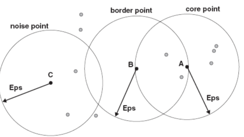
Core points are in the interior of a density-based cluster.
A point is a core point if the number of points within or at the boundary of a given neighborhood of the point is greater than or equal to a certain threshold MinPts.
The size of the neighborhood is determined by the distance function and a user-specified distance parameter, Eps.
The threshold MinPts is also a user-specified parameter.
In the figure on slide 30, A is a core point for the indicated radius (Eps) if MinPts=7.
A border point is not a core point, but falls within or at the boundary of the neighborhood of a core point.
In the figure on slide 30, B is a border point.
A border point can fall within the neighborhoods of several core points.
A noise point is any point that is neither a core point nor a border point.
In the figure on slide 30, C is a noise point.
While there are points which have not been processed:
For one of these points, check whether it is a corepoint or not.
If it is not a core point
- Label it as a noise point (This label may change later).
If it is a core point, label the point and
- Form a new cluster Cnew using this point.
- Include all points within or at the boundary of its Eps-neighborhood, which have not been previously assigned to a cluster, in Cnew.
- Insert all these neighboring points into a queue.
- While the queue is not empty,
  - Remove the first point from the queue.
  - If this point is not a core point, label it as a border point.
  - If this point is a core point, label it and check every point within or at the boundary of its Eps-neighborhood which was not previously assigned to a cluster.
  - For each of these unassigned neighboring points,
    - Assign the point to Cnew.
    - Insert the point into the queue.
The left figure on the next slide shows a sample data set with 3000 2-D points.
The right figure shows the resulting clusters found by DBSCAN.
The core points, border points and noise points are also displayed.